Voronoi diagrams of polygonal objects
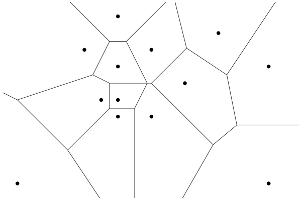
We investigate problems on generalized Voronoi diagrams of polygonal objects in Euclidean space \(\mathbb{R}^d\). Voronoi diagrams are among the most fundamental structures in Computational Geometry and they have proved powerful tools in solving diverse computational problems. The standard Voronoi diagram of a set of sites is a subdivision of the plane into regions such that the Voronoi region of a site p is the locus of points closest to p than to any other site. Sites can be points, polygonal objects, or other types of geometric objects. Higher order Voronoi diagrams encode k-nearest neighbor information and they define a partitioning of space into maximal regions such that every point within a region has the same k nearest sites.
Our project is funded by SNF (under project number 127137).
Gaussian map
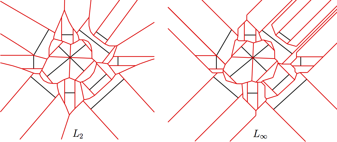
The Gaussian map encodes information about the unbounded cells of a Voronoi diagram. This structure is of particular interest when all cells are unbounded. For example, all the d-dimensional cells of the farthest Voronoi diagram of segments or lines are unbounded. Roughly speeking, the Gaussian map is the intersection of the diagram with a big circle / hypersphere.
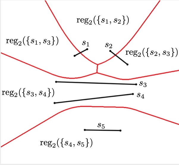
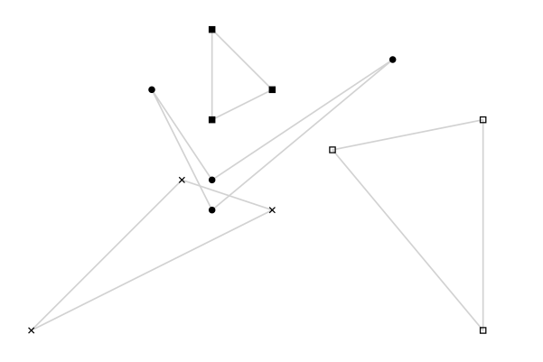
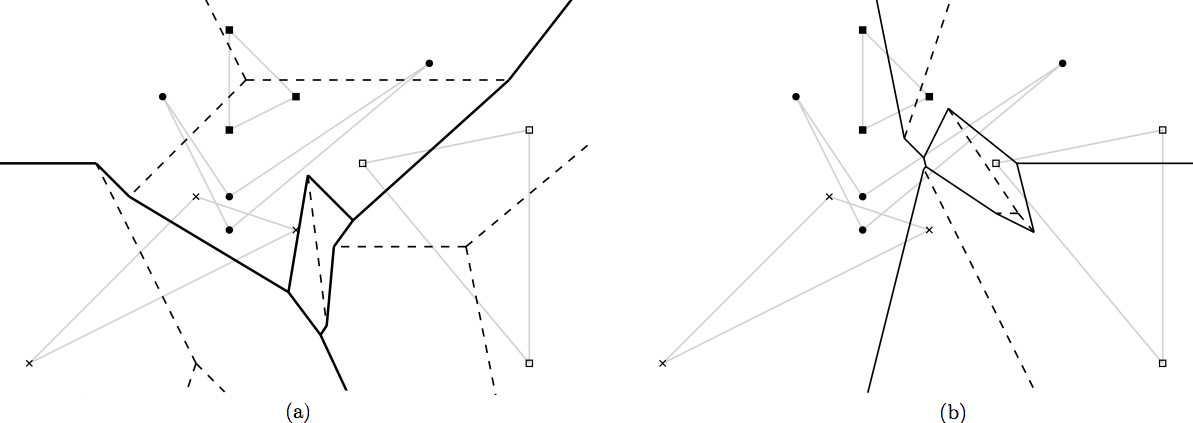
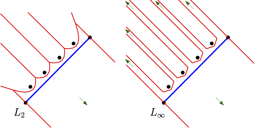
An order-2 Voronoi diagram of 5 segments in 2D
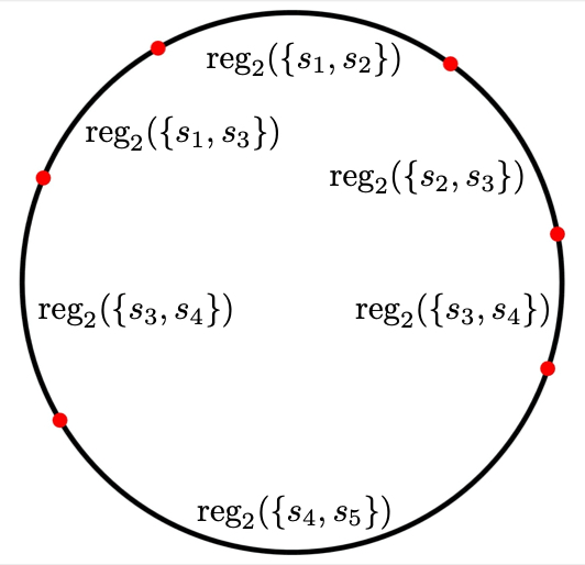
and its Gaussian map.
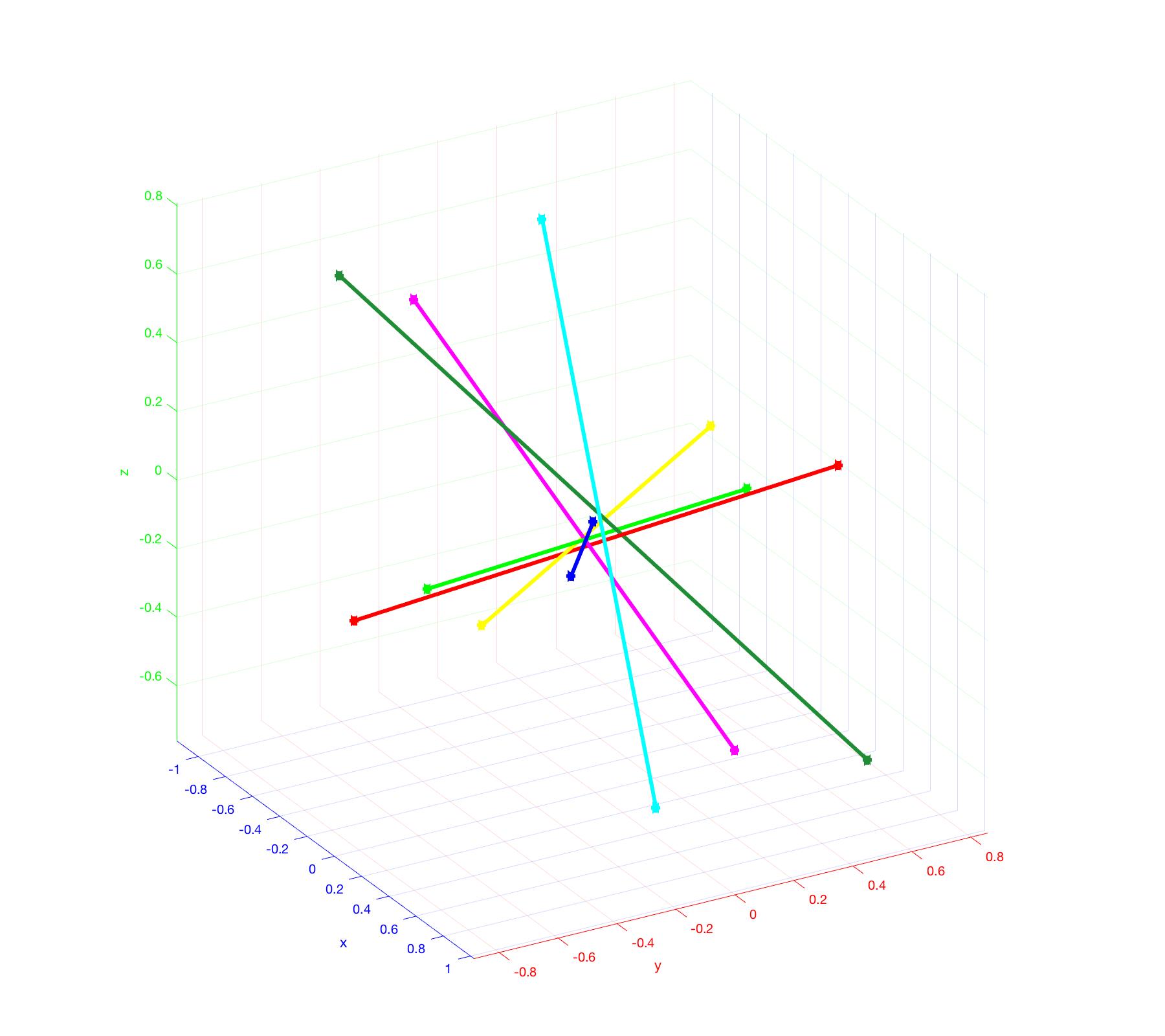
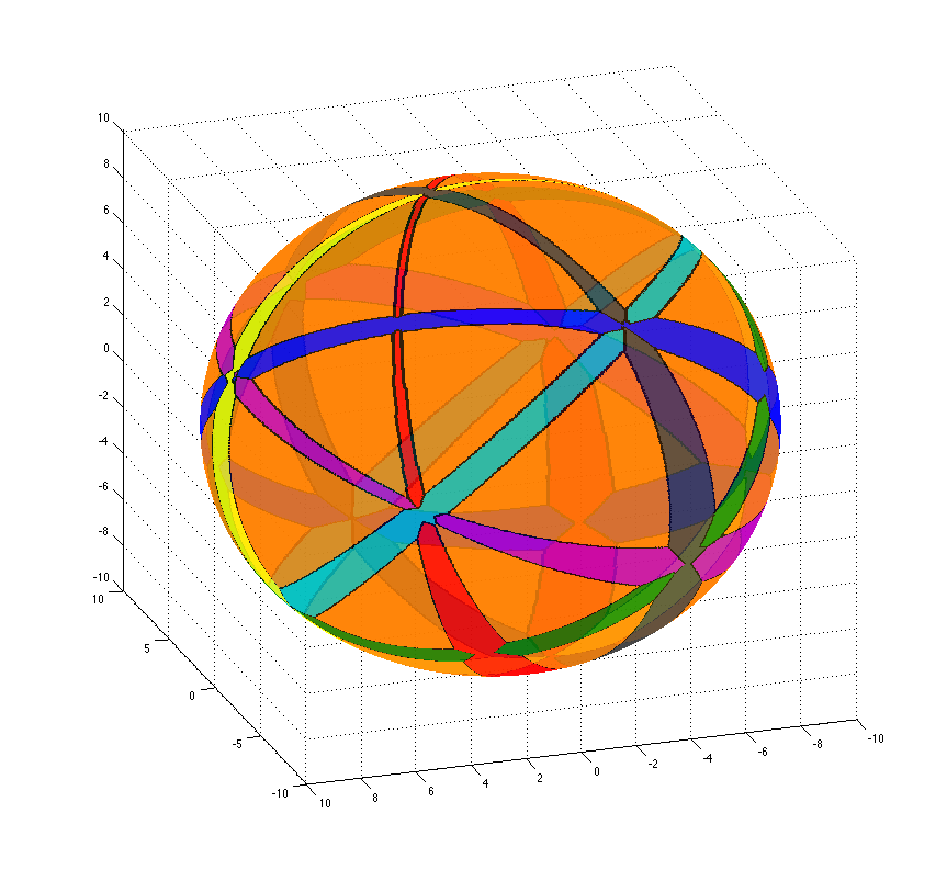
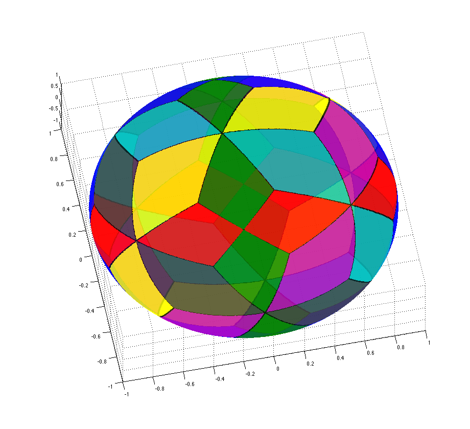
Segments in 3D
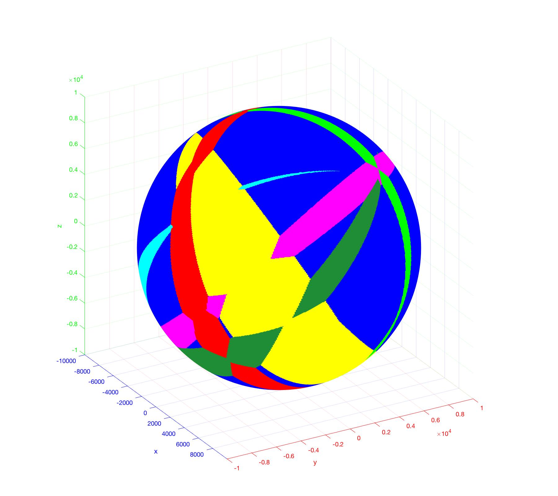
and the Gaussian map of their farthest Voronoi diagram.
The Gaussian map of the order-k Voronoi diagram of n lines or line segments in \(\mathbb{R}^d\) has \(O(\min\{k, n-k\} n^{d-1})\) complexity, which for \(k=n-1\) is tight in worst-case. It can be computed in \(O(n^{d-1} \alpha(n))\) time.
Visualization of the collapse algorithm for 4 segments in 2D. The farthest region of each segment is colored in the same color as the segment itself.
The trisector of three segments (one segment has 0 length) in 3D can be a closed curve. The distance of a point on the trisector to the segments is encoded by colors (blue = small distance, yellow = big distance).
The trisector of 3 lines in 3D. The distance from a point on the trisector to the lines is encoded by colors (small distance = red -> orange -> yellow -> green -> blue = big distance). The distance function restricted to the middle branch of the trisector induces a local maximum (walking along the branch the colors change from ... -> orange -> yellow -> orange -> ...).
Hausdorff and higher order Voronoi diagrams
Spacial Decompositions and Graphs (short nickname: VORONOI) is a collaborative research project. It involves 8 partners from 6 different countries, and it is part of the EuroGIGA program of the European Science Foundation (ESF).
Our group, in particular, investigates problems related to Hausdorff and higher-order Voronoi diagrams in the plane. The objective is to derive a deeper understanding of these fundamental geometric structures, link them with the existing theoretical framework, and produce efficient but simple algorithms for their construction. Diverse application areas can directly benefit from such algorithms. An example is the area of VLSI yield analysis and design manufacturability (DFM), where generalized Voronoi diagrams of polygonal objects have already provided the basis of most advanced design automation tools in the semiconductor industry.
Our individual subproject is funded jointly by SNF (under project number 134355) and ESF.
Cluster Voronoi diagrams
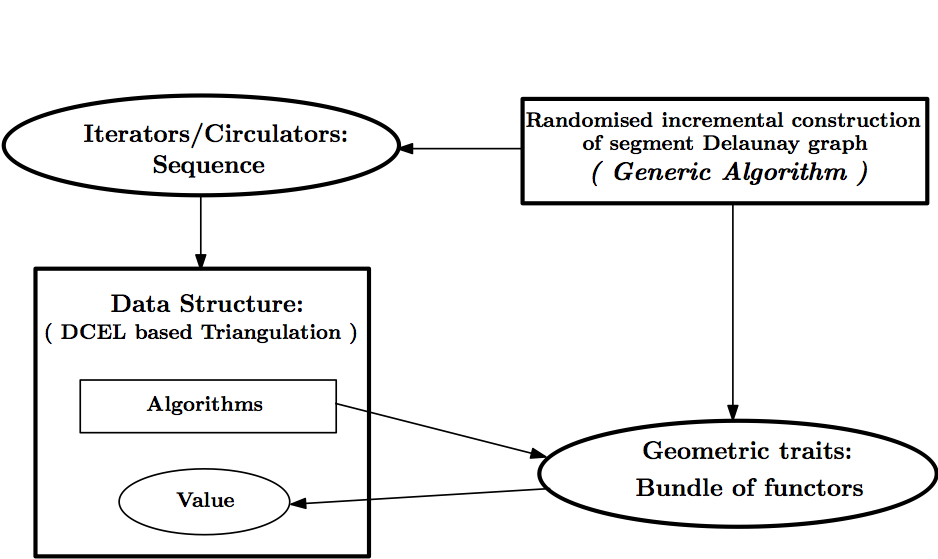
CGAL implementation
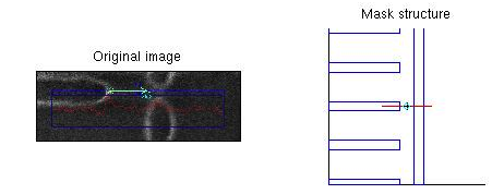
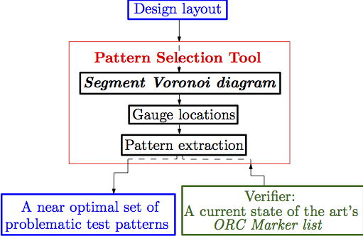
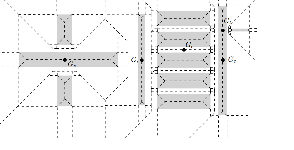
VLSI pattern analysis
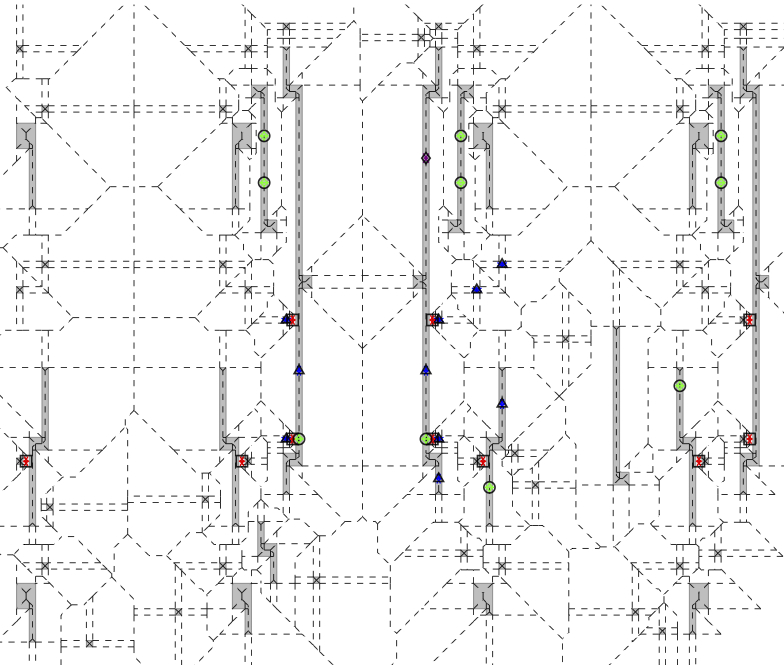
Box Subdivision algorithms
A classic problem in Facility Location is to place a facility in order to serve a given set of demand points or customers such that it minimizes the total transportation costs. The total cost at any point is interpreted as the sum of the distances to the demand points. The point that minimizes this sum is called the Fermat Point. This is an old geometric problem that has inspired scientists over the last three centuries.
A foci set is a non-empty finite set of (demand) points \(X = \{a_1,...,a_k\}\). The Fermat distance function is given by \(\phi(x) = \sum_{a \in X} ||x-a||\). The global minimum \(r^* = \min_{x \in \mathbb{R}^d} \phi(x)\) is called the Fermat radius; any point x that achieves this minimum, is called a Fermat point.
We also consider the closely related problem of computing \(k\)-ellipses of \(X\). For any \(r>r^*(X)\), the level set of the Fermat distance function is \(\phi^{-1}(r) = \{x \in \mathbb{R}^d: \phi(x)=r\}\). If \(k=1\), this level set is a sphere; if \(k=2\), the level set is the classic ellipse if \(d=2\). When \(X\) has \(k\) points, we call \(\phi^{-1}(r)\) a \(k\)-ellipsoid, or \(k\)-ellipse in the planar case. We want to approximate such \(k\)-ellipses, viewed as curves that bound the set of facility locations whose total transportation cost is at most some specified \(r\). More generally, we might want to simultaneously approximate several such \(k\)-ellipes.
See our EuroCG 2020 paper for more details and references. Click here for watching a video that summerizes the most important parts of this paper.
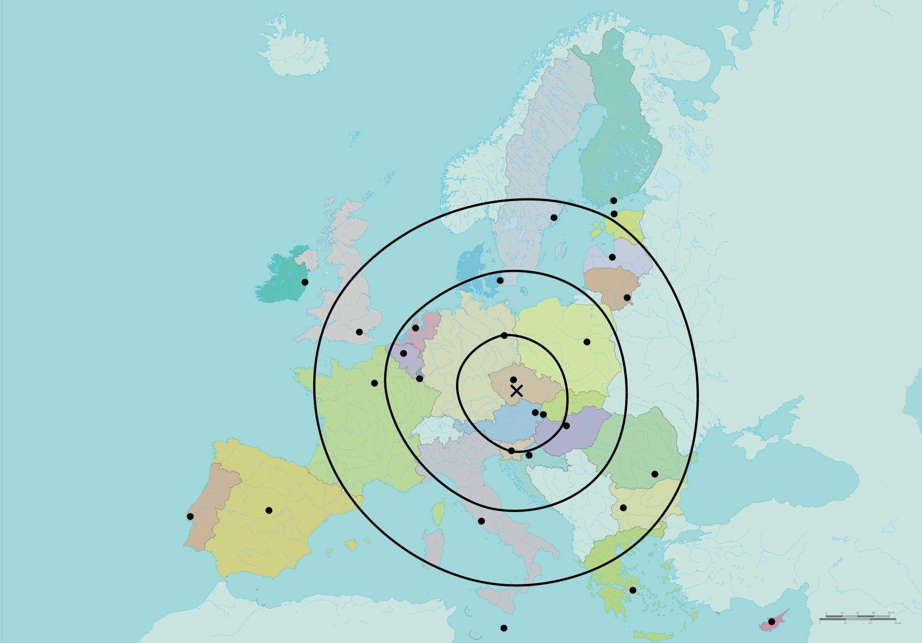 The Fermat point of the capitals of Europe marked with \(\times\). Moreover, three 28-ellipses are plotted. The original map was taken from https://www.consilium.europa.eu.
Box subdivision algorithm finding the Fermat point.
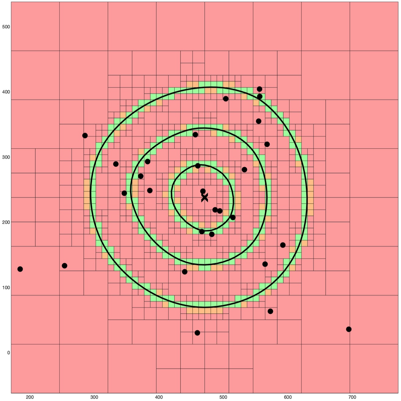
Box subdivision for computing the 28-ellipses of 3 radii.
Visualization of the pointsequence, which converges to the Fermat point, and also the boxes involved in the tests.
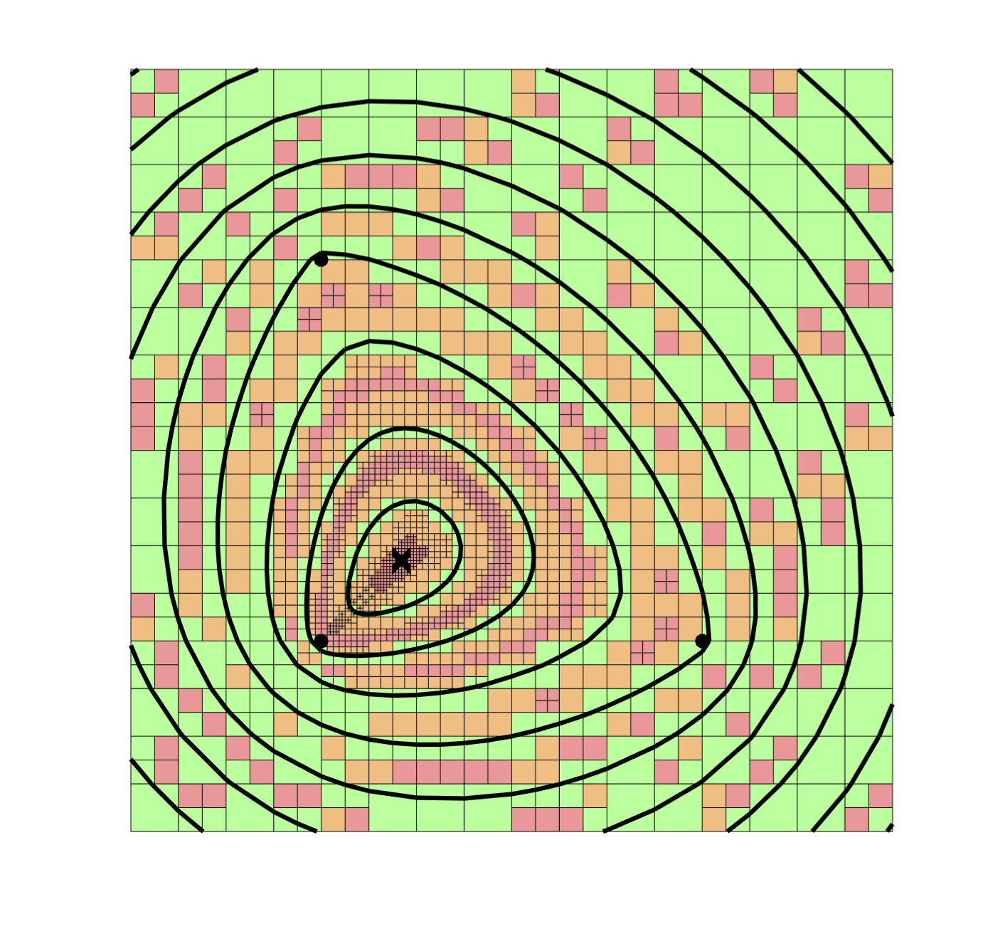 A contour plot of 3 foci and with 10 different radii.